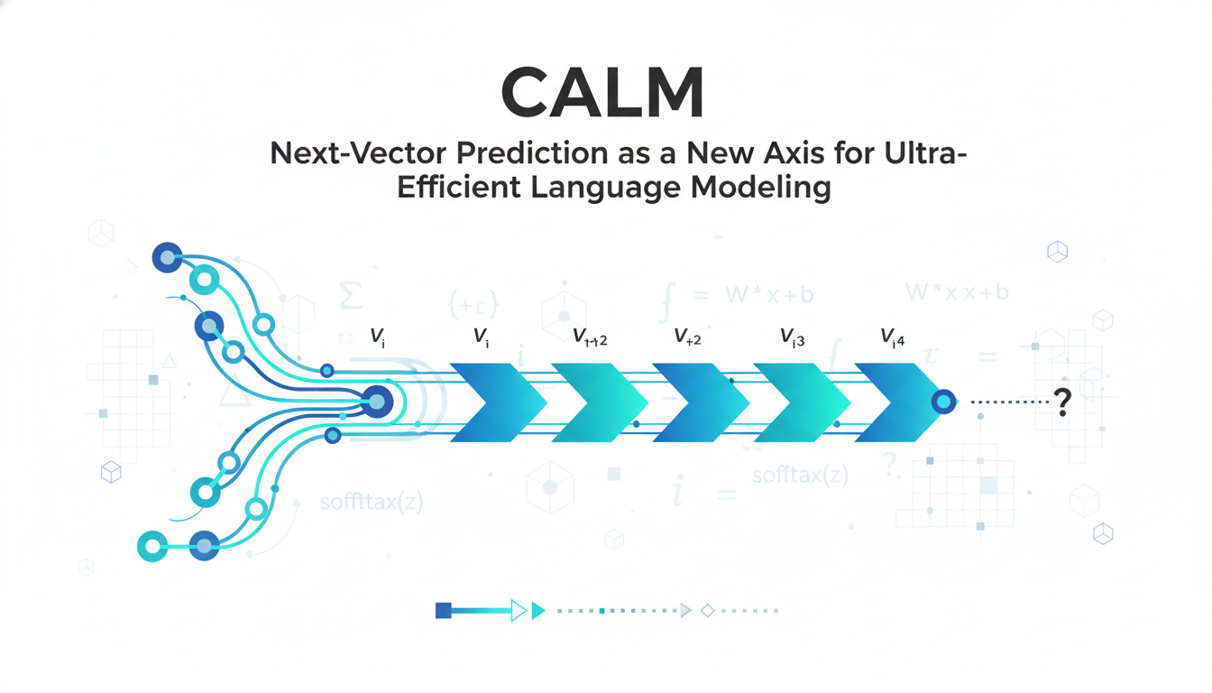
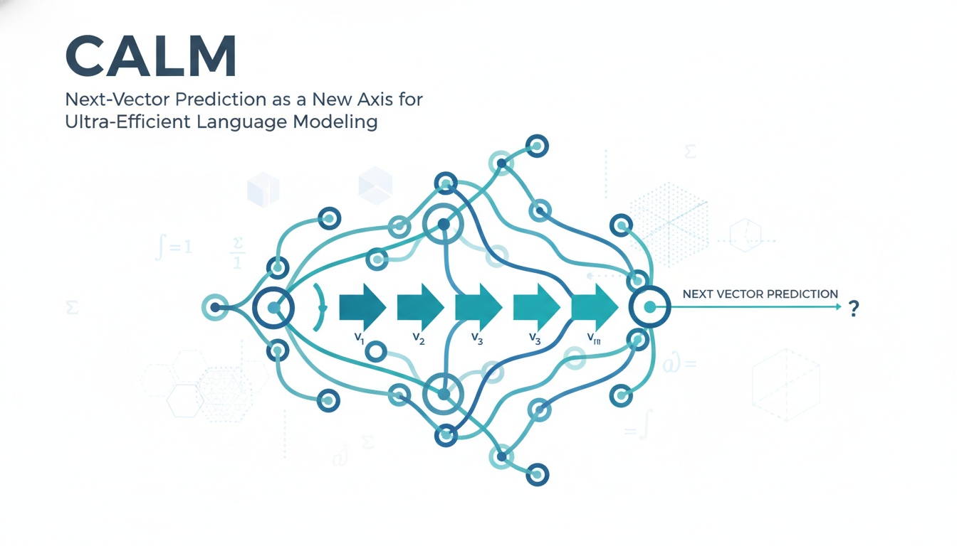
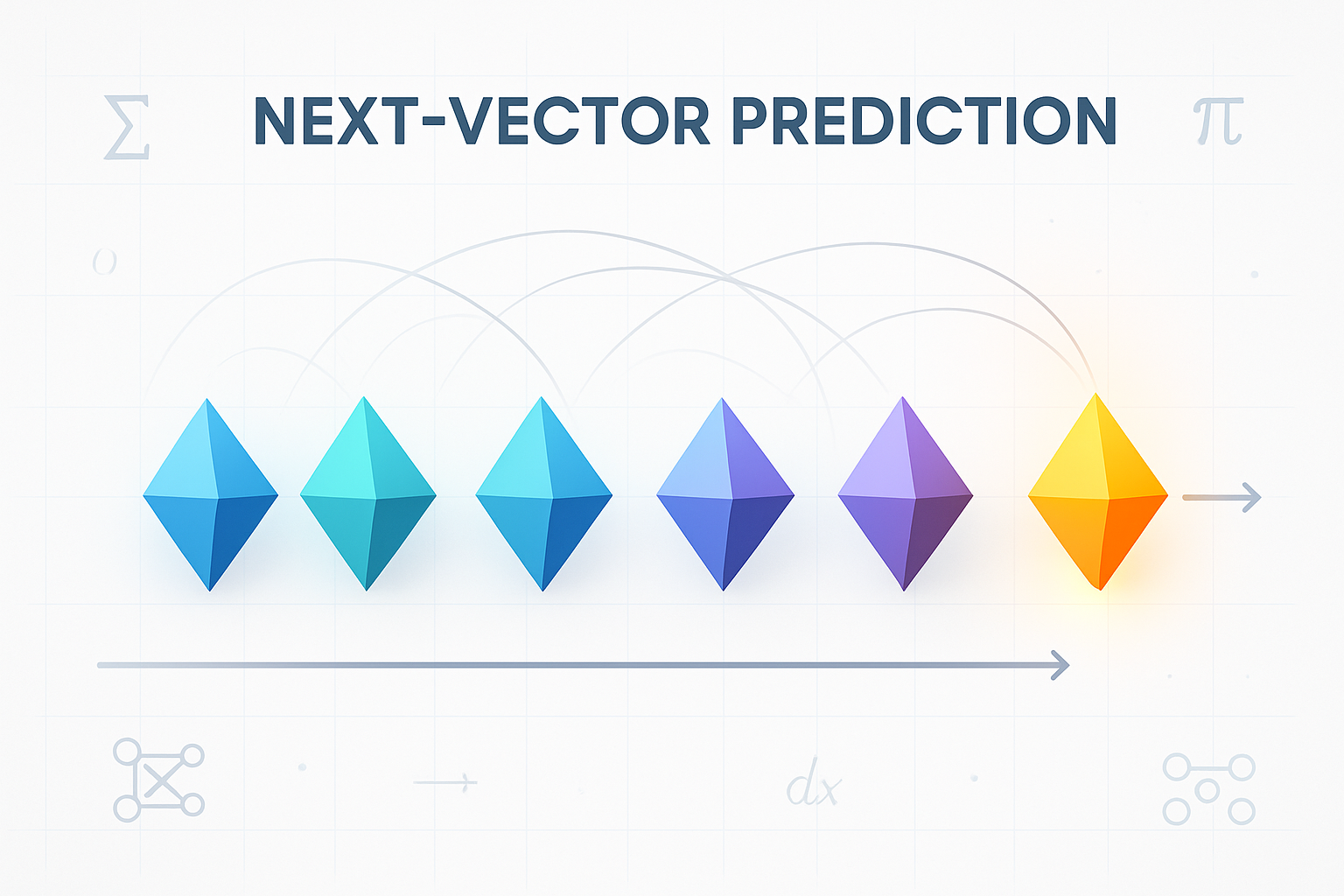
Continuous Autoregressive Language Models - Full Paper and Review

What if we stopped predicting the next token—and predicted the next vector instead? That’s the central shift proposed by Continuous Autoregressive Language Models (CALM), a framework that compresses chunks of tokens into continuous vectors, models those vectors autoregressively, and decodes them back to text with striking fidelity. Rather than speeding up token-by-token generation with clever engineering, CALM widens the data “pipe” per step—increasing the semantic bandwidth of each generative move—so you take fewer steps overall.

CALM pairs a lightweight but high-fidelity autoencoder with a likelihood-free generative head and an evaluation toolkit tailored to the continuous domain. The result is a performance–compute frontier that, in the authors’ experiments, outperforms comparable Transformers on total FLOPs for both training and inference at similar quality levels.

If you want to skim the originals, the authors link to their code and project page right up front.

CALM Download

Why CALM?

Modern LLMs are still bottlenecked by sequential next-token generation: they must take one step per token, and long contexts or outputs imply many steps—and much compute. The CALM paper argues for a new scaling axis: make each step carry more meaning. Concretely, CALM compresses K tokens → 1 vector, then predicts the next vector instead of the next token, cutting the number of autoregressive steps by roughly a factor of K.

This is more than an incremental trick. It reframes language modeling as next-vector prediction on a continuous sequence, not a discrete one, and that shift has deep implications for modeling, evaluation, and sampling.

The CALM Pipeline, in One Picture

At a high level, each generation step proceeds as follows:

Encode the last K tokens into a continuous vector z with a compact autoencoder.
Condition a Transformer backbone on the compressed history (discrete tokens are fed through an input-compression MLP).
Sample the next latent z from a generative head (an energy-based, single-step module).
Decode z back to K output tokens, append them, and repeat.

In the authors’ schematic (Figure 2), the Transformer backbone outputs a hidden state hhh, while the generative head refines a noise vector through residual MLP blocks (with SwiGLU activations) into the predicted latent zzz. A lightweight decoder then maps zzz back to tokens for the next step.

One empirically crucial detail: feed discrete tokens—not latent vectors—into the Transformer. Using previous latents as inputs looked attractive, but degraded performance because the model struggled to unpack so much compressed meaning. The authors instead compress token embeddings with an input-compression MLP, which maintained quality.

A Tiny but Mighty Autoencoder

CALM’s autoencoder is designed to be small, fast, and accurate:

Encoder: map x1:Kx_{1:K}x1:K to K embeddings → per-position FFN → flatten → linear compression RKd→Rd\mathbb{R}^{K d} \to \mathbb{R}^{d}RKd→Rd → FFN → linear to latent dimension lll.
Decoder: linear + FFN → expand to KdK dKd → reshape to K states → per-position FFN → projection to vocabulary logits → argmax tokens.

Despite being shallow (hidden size d=512d=512d=512), the autoencoder can be extremely compact. With K = 4, a latent of just l=10l=10l=10 achieves >99.9% token-level reconstruction accuracy—and the module’s compute overhead is “nearly negligible” compared to the LM.

Making the Latent Space Robust (and Why That Matters)

A reconstruction-only autoencoder will “pack” information densely in a brittle way. Tiny perturbations in zzz can decode to entirely unrelated text—fatal for generative modeling that must traverse latent space step by step. The authors therefore regularize the latent manifold to make it smooth and robust.

They move from a deterministic AE to a variational one: the encoder outputs (μ,σ)(\mu,\sigma)(μ,σ) of a diagonal Gaussian, adding a KL term against a standard normal prior with a small weight (β=0.001\beta=0.001β=0.001). This discourages extreme or overly precise latent codes and smooths the manifold.

To counter posterior collapse, they clip each dimension’s KL at a floor (λKL=0.5\lambda_{KL}=0.5λKL=0.5) so all dimensions carry information (preventing “dead” latents that inject noise). And they add dropout in two places: randomly mask input tokens (p=0.15) and drop pieces of the latent vector zzz (p=0.15). The combination forces redundancy and boosts robustness to the small prediction errors inevitable in generation.

In ablations, the remedy is clear: naive VAE hurts via collapse; KL clipping fixes it; token-dropout and latent-dropout deliver complementary gains.

The Generative Head: Likelihood-Free, Single-Step, Energy-Based

Since CALM lives in a continuous vector space, the usual softmax over a discrete vocabulary vanishes. That removes direct likelihoods—and with them, familiar tools like cross-entropy and temperature-scaled logits. The authors lean into this with a likelihood-free generative strategy.

They deliberately avoid diffusion and flow-matching heads, which require many iterative steps per vector (undoing the speedups CALM seeks). Instead, they adopt an Energy Transformer head optimized with a strictly proper scoring rule—the energy score—which supports single-step generation and can be trained from samples alone.

A proper scoring rule’s expected score is maximized when the predictive distribution matches the data distribution; a strictly proper rule uniquely identifies the truth. This generalizes maximum-likelihood training (which relies on the logarithmic score) into the continuous domain where likelihoods are intractable.

The energy score measures sample-distance alignment between predictions and ground truth and admits a Monte Carlo energy loss. In practice, they draw N candidate samples from the head and M target samples from the autoencoder’s conditional posterior to stabilize the estimate (they use N = 8 and M = 100).

Architecture-wise, the head is just a stack of residual MLP blocks (with SwiGLU), fusing the Transformer’s hidden state hhh with a noise vector ε\varepsilonε. It contributes only ~10% of total parameters—minimal overhead for the backbone.

Evaluating Without Likelihoods: BrierLM

Perplexity goes out the window if we can’t compute probabilities. CALM introduces BrierLM, a likelihood-free evaluation metric adapted from the classic Brier score, which balances accuracy and uncertainty calibration. Key insight: the Brier score can be estimated from samples alone, using collisions between independent draws.

Concretely, draw two independent samples x1,x2x_1,x_2x1,x2 from the model and compare them with the ground truth yyy. The unbiased estimator of the Brier score is
I{x1=y}+I{x2=y}−I{x1=x2}\mathbb{I}\{x_1 = y\} + \mathbb{I}\{x_2 = y\} – \mathbb{I}\{x_1 = x_2\}I{x1=y}+I{x2=y}−I{x1=x2}. Summed over n-grams (for n=1..4) and geometrically averaged, this yields BrierLM on a 0–100 scale. It applies to standard Transformers too (by sampling from their softmax), enabling fair comparisons across modeling paradigms.

Temperature Sampling—Without Logits

How do you do temperature sampling (control randomness) when you don’t have logits? CALM contributes a clever rejection-sampling algorithm that transforms a black-box sampler into samples from the temperature-adjusted distribution PT(x)∝P(x)1/TP_T(x) \propto P(x)^{1/T}PT(x)∝P(x)1/T.

The core idea: when T=1/nT = 1/nT=1/n is the reciprocal of an integer, the probability of drawing the same outcome in n independent draws is P(x)nP(x)^nP(x)n. So: draw n samples; accept them only if all n are identical. The accepted outputs are distributed proportionally to P(x)nP(x)^nP(x)n, i.e., the target temperature law. The general algorithm handles non-integer 1/T1/T1/T with a two-stage procedure (integer part, then a fractional part).

The authors analyze the expected number of sampler calls and show explicit bounds. Practical takeaway: avoid temperatures too close to 1 (can scale with sample-space size) and very low temperatures (high rejection from requiring many identical draws). They therefore also provide an efficient batch approximation tailored to low temperatures T=1/nT=1/nT=1/n: draw a large batch, count nnn-tuples of matching samples combinatorially, and pick among candidates with weights equal to the number of combinations. It’s biased for finite batches but asymptotically unbiased as batch size grows.

Pseudocode lovers will appreciate the clarity of Algorithm 1 (exact) and Algorithm 2 (approximate) in the paper.

Experimental Setup (at a Glance)

Training proceeds in two stages:

Autoencoders are trained on a 15B-token subset of The Pile for chunk sizes K∈{1,2,4,8}K\in\{1,2,4,8\}K∈{1,2,4,8}. They’re tiny: hidden size 512, latent dimension 32K32K32K, about 75M parameters, trained for 30k steps with batch size 512k tokens.
CALM models are then trained on the remaining data for 250k steps with batch size 2M tokens. Context length is 2048 steps (for CALM that’s 2048K2048K2048K tokens). Optimization uses AdamW with typical settings (β1_11=0.9, β2_22=0.95, etc.).

Results: A New Performance–Compute Frontier

The headline comparison (with K=4) shows CALM achieving comparable or better BrierLM at substantially lower FLOPs. For example:

Transformer-S (281M) vs CALM-M (371M, K=4):
CALM-M matches or surpasses the baseline BrierLM while needing 44% fewer training FLOPs and 34% fewer inference FLOPs.

The full table (including L and XL scales) reports parameters, training/inference FLOPs, and BrierLM, and notes that CALM’s FLOP/param counts include the autoencoder’s overhead. Attention FLOPs are computed at context length 2048.

The “Semantic Bandwidth” Knob (K)

Beyond scaling parameters, CALM introduces K as a design knob. On the authors’ CALM-L curve:

Moving from K=1 → K=2 almost halves the cost with only a marginal performance dip.
At K=4, CALM surpasses the discrete baseline’s performance–compute frontier.
At K=8, performance drops more sharply—likely a capacity limit for the tested model sizes, suggesting larger backbones could better leverage higher K.

This is the paper’s central message in action: scale the information per step, not only the number of parameters and data.

Ablations: What Actually Mattered

Autoencoder regularization made or broke the system:

Naive VAE: big drop (posterior collapse).
KL clipping: crucial fix (prevents dimensions from becoming pure noise).
Dropout (tokens + latent): consistent, orthogonal gains.
KL weight β: small β helps smooth the manifold with negligible impact on reconstruction, but overly large β harms both reconstruction and downstream BrierLM. The authors settle on β = 0.001.

They also sweep latent dimension lll and adjust dropout correspondingly (e.g., higher lll → higher dropout rate) to balance capacity and robustness; figures in the paper chart the trade-offs between reconstruction accuracy and BrierLM.

Why BrierLM and Energy Loss Are a Good Fit

The Brier score is a classic, strictly proper scoring rule that rewards calibrated predictions, not just accurate ones. Its decomposition shows a squared-error term minimized at the true distribution plus a constant data-variance term—so maximizing it aligns the model’s predictive distribution with reality. Crucially, the collision-probability trick lets CALM estimate Brier from samples alone, bridging the evaluation gap in a likelihood-free setup.

On the training side, the energy score (another strictly proper rule) yields an energy loss computable via Monte Carlo sampling. Combining multiple model draws NNN with multiple “target” samples MMM from the autoencoder’s conditional Gaussian posterior stabilizes the gradient signal—pragmatic and effective.

Together, BrierLM + energy loss form a principled pair for learning and measuring in a world without explicit likelihoods.

Temperature, in Practice

Without logits, temperature becomes an algorithmic problem: how to transform a sampler for PPP into a sampler for PTP_TPT. CALM’s exact algorithm is correct but can be costly at very high or very low temperatures. The authors therefore recommend avoiding extremes and provide a batch approximation that’s simple to implement and asymptotically unbiased. The approximation reframes “draw n identical samples” as “find n-tuples inside a batch,” draws a weighted candidate, and falls back to smaller nnn if necessary so it always returns a result.

If you’ve ever wanted temperature control in a non-softmax generator, this section is a gem.

Limitations and Open Questions

The paper is refreshingly candid about the trade-offs:

K too small (e.g., 1): CALM pays a penalty; continuous prediction is harder than discrete next-token, so you lose compute/perf ground compared to a standard Transformer until K grows.
K too large (e.g., 8): performance drops unless the model is scaled up—suggesting a capacity mismatch.
Exact temperature sampling can be inefficient at certain temperatures; the approximate scheme is recommended in low-temperature regimes.

There’s also an architectural nuance: use discrete tokens as inputs, not latents, to avoid forcing the backbone to unpack too-dense signals. That empirical finding hints at interesting future hybrids for conditioning and context compression.

Why CALM Matters

CALM is best understood as a design axis rather than a single model: keep your familiar Transformer backbone, but turn up the semantic bandwidth per autoregressive step. When done carefully—with robust latents, a single-step generative head, and likelihood-free training/evaluation—this opens a path toward ultra-efficient LLMs that do competitive work with fewer total FLOPs.

In the authors’ results, CALM-M (371M) essentially meets a Transformer-S (281M) on quality with far fewer training and inference FLOPs—including the autoencoder’s full overhead. That’s not a cherry-picked microbenchmark; it’s a table with careful accounting and a new metric (BrierLM) designed to compare continuous and discrete models fairly.

Beyond immediate wins, CALM reframes how we might scale models over the next few cycles. Just as moving from characters to subword tokens compressed sequences and unlocked the Transformer era, the move from tokens to continuous vectors may enable the next set of efficiency leaps—especially as we push output lengths, context windows, and multimodal streams upward.

How to Explore Further

Code: The authors publish their implementation here: github.com/shaochenze/calm.
Project Page / Write-up: A concise overview with figures and intuition: Project page.
Background reading:
- Brier score (calibration): see the derivation and the collision-probability estimator in the paper’s Section 4.
- Energy score and strictly proper scoring rules: Section 3.3.

TL;DR (for busy builders)

What’s new: Model the sequence as continuous vectors; predict the next vector instead of the next token. Cut steps by K via chunking, then decode back to text.
How it works: A tiny autoencoder (accurate, robust via VAE + KL-clipping + dropout)
Why it matters: Introduces semantic bandwidth (K) as a new lever for performance–compute optimization. With K=4, CALM beats the Transformer baseline frontier on FLOPs at similar quality—even counting autoencoder overhead.
Caveats: K must match model capacity; exact temperature sampling can be costly at extremes (use the batch approximation).

Closing Thoughts

CALM isn’t a repudiation of the Transformer; it’s a reinterpretation of its generative loop. By compressing K tokens into one latent, adding just enough structure and noise to make that latent space navigable, and then generating in one shot per chunk, CALM advances a serious alternative to “faster softmax” thinking. It’s a bet that efficiency gains lie not only in better kernels, quantization, or caching, but in changing the unit of prediction itself. And on the evidence presented—metrics, algorithms, ablations, and compute accounting—it’s a compelling bet.

If you’re building systems that care about throughput per watt and latency at long outputs, CALM’s recipe is well worth studying—and perhaps, soon, adopting.